Previously, we have explored methods to compute the essence of power functions $Ȣx^n$ which involves solving a large system of linear equations. This method is equivalent to solving for the inverse of a large $n\times n$ matrix where entries are values of pascal's triangle. Though the matrix method allow us to solve for large number of essences at once, it does not extend easily to solve for next iterations of essence coefficients. Rather than reusing the values we have already solved for, we will have to solve for inverse of a separate larger matrix again. Here we will introduce an iterative method for solving for these coefficients. Chapter 0: Recap Let us first remind ourselves of the definition of essence. For a function $f(x)$, we want to find the transformation $Ȣf(x)$ such that we are able to 'smooth out' its series: $$\sum_{i=a}^b f(i) = \int_{a-1}^b Ȣf(x) dx$$ For example, we can solve for the following functions: $$\begin{align*}Ȣ1 &= 1 \\ Ȣx &= x +...
Previously, we have explored methods to compute the essence of power functions $Ȣx^n$ which involves solving a large system of linear equations. This method is equivalent to solving for the inverse of a large $n\times n$ matrix where entries are values of pascal's triangle.
Though the matrix method allow us to solve for large number of essences at once, it does not extend easily to solve for next iterations of essence coefficients. Rather than reusing the values we have already solved for, we will have to solve for inverse of a separate larger matrix again.
Here we will introduce an iterative method for solving for these coefficients.
Interestingly, the essence transformation seems to preserve the overall 'form' of the function it is transforming. Note even on the short list of examples above, n-degree polynomial transforms to be another n-degree polynomial. Looking into systems of equations method of solving for these essence, we can see that this should hold true. In general, for power functions the transformation yields polynomial of form $$\begin{align*} Ȣx^n &= b_{n}^{(n)} x^n + b_{n-1}^{(n)}x^{n-1} + \dots + b_{1}^{(n)}x + b_{0}^{(n)} \\ &= \sum_{i=0}^{n} b_{i}^{(n)} x^{i} \end{align*}$$ where we will call $b_{i}^{(n)}$ the $i$th essence coefficient for $n$th power.
Our goal now becomes solving for these coefficients easily.
Assuming that the previous power $Ȣx^{n-1}$ is known, $$\begin{align*} \because Ȣx^{n-1} &= \sum_{j=0}^{n-1} b_{j}^{(n-1)} x^{j} \\ \therefore Ȣ\int x^{n-1} dx &= \int Ȣx^{n-1} dx + c \\ &= \int \sum_{j=0}^{n-1} b_{j}^{(n-1)} x^{j} dx \, + c \\ Ȣ \frac{1}{n}x^n &= \sum_{j=0}^{n-1} \int b_{j}^{(n-1)} x^{j} dx \, + c \\ &= \sum_{j=0}^{n-1} \frac{b_{j}^{(n-1)}}{j+1} x^{j+1} \,+ c \\ &= \sum_{i=1}^{n} \frac{b_{i-1}^{(n-1)}}{i} x^{i} + c \\ \therefore Ȣ x^n &= \sum_{i=1}^{n} \left(n\frac{b_{i-1}^{(n-1)}}{i}\right) x^{i} \,+ c' \end{align*}$$ By following each coefficients found here, we can see that for all non-constants' coefficients $$\begin{align*} & b_{i}^{(n)} = \frac{n}{i}b_{i-1}^{(n-1)}, & 1\leq i \leq n \end{align*}$$ This still leaves us $b_{0}^{(n)}$ to be solved.
These $b_{0}^{(n)}$ are in fact the $n$th Bernoulli Numbers. To solve for the $b_0^{(n)}$, we return to the definition for essence. We want the found $Ȣx^n$ to statisfy $$\sum_{i=a}^b x^n = \int_{a-1}^b Ȣx^n dx$$ For instance, for $a=b=k$ $$\begin{align*} k^n &= \int_{k-1}^k Ȣx^n dx \\ &= \int_{k-1}^k \sum_{i=0}^{n}b_{i}^{(n)}x^i dx \\ &= \left. \sum_{i=0}^n \frac{b_{i}^{(n)}}{i+1}x^{i+1} \right|_{k-1}^k \end{align*}$$ Namely, for when $k=1$, we see that the equation simplifies to $$1 = \sum_{i=0}^{n} \frac{b_{i}^{(n)}}{i+1}$$ Thus, once we have found all the non-constants' coefficients, we can solve for the final constant by $$b_0^{(n)} = 1 - \sum_{i=1}^{n} \frac{b_{i}^{(n)}}{i+1} $$
Here we notice another interesting fact.
For when $k=0$, $$\begin{align*} 0 &= \sum_{i=0}^{n} (-1)^i \frac{b_{i}^{(n)}}{i+1} \\ &= \sum_{i \text{ Even}} \frac{b_{i}^{(n)}}{i+1} - \sum_{i\text{ Odd}} \frac{b_{i}^{(n)}}{i+1} \end{align*}$$ $$\therefore \sum_{i \text{ Even}} \frac{b_{i}^{(n)}}{i+1} = \sum_{i\text{ Odd}} \frac{b_{i}^{(n)}}{i+1} $$ Combined with the previous result that sum of all of these terms equal 1, we find that these even and odd sums must individually equal half. $$\sum_{i \text{ Even}} \frac{b_{i}^{(n)}}{i+1} = \sum_{i\text{ Odd}} \frac{b_{i}^{(n)}}{i+1} = \frac{1}{2}$$ This fact becomes very useful later on.
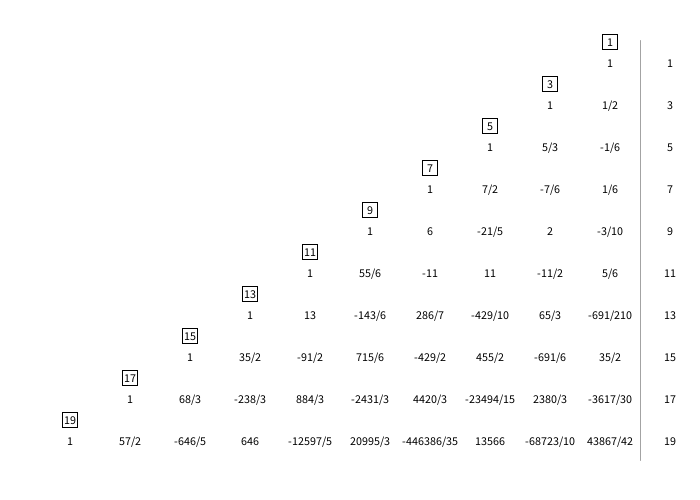
Then we are able to draw the following table. The $b_{i}^{(n)}$ is written in black and $\frac{b_{i}^{(n)}}{i+1}$ is written in red under the corresponding term.
Above the $i$th column, $i+1$ is written in a circle to help with solving for intermediate terms in red.
To the right of each row, $n$ is written.
The generation progress is visualized step by step: Following this process, we can arrive at a larger table such as this:
 Just by knowing the previous iteration, we are able to solve for the next layer of coefficients, making this method more preferable to the matrix inverse method.
With this table laid out, we are able to notice some interesting patterns. Most glaring is that $b_{0}^{(n)} = 0$ for all odd $n > 1$. We will now prove this fact.
For example $$\begin{align*} \sum_{i=0}^x i^0 &= 1x \\ \sum_{i=0}^x i^1 &= \frac{1}{2}x^2 + \frac{1}{2}x \\ \sum_{i=0}^x i^2 &= \frac{1}{3}x^3 + \frac{1}{2}x^2 + \frac{1}{6}x \\ \sum_{i=0}^x i^3 &= \frac{1}{4}x^4 + \frac{1}{2}x^3 + \frac{1}{4}x^2 + 0x \\ \sum_{i=0}^{x} i^{4} &= \frac{1}{5}x^5 + \frac{1}{2}x^4 + \frac{1}{3}x^3 + 0x^2 - \frac{1}{30}x \\ &\vdots \end{align*}$$
$b_{n}^{(n)} = 1$ following $$\begin{align*} \because b_{0}^{(0)} &= 1 \\ b_{n}^{(n)} &= \binom{n}{n}b_{0}^{(0)} \\ &= 1 \end{align*}$$ $\frac{b_{n-1}^{(n)}}{n} = \frac{1}{2}$ following $$\begin{align*} \because b_{0}^{(1)} &= \frac{1}{2} \\ \frac{1}{n}b_{n-1}^{(n)} & = \frac{1}{n}\binom{n}{n-1}b_{0}^{(1)} \\ &= \frac{n}{n}\frac{1}{2} \\ &= \frac{1}{2} \end{align*}$$ With these and previous results, we are ready to prove that every odd bernoulli number must be zero.
For $2m+1 \geq 3$ $$\begin{align*} b_{0}^{{2m+1}} &= 1 - \sum_{i=1}^{2m+1} \frac{1}{i+1}b_{i}^{(2m+1)} \\ &= 1 - \sum_{\substack{i=1\\ i\text{ Odd}}}^{2m+1} \frac{1}{i+1}b_{i}^{(2m+1)} - \sum_{\substack{i=1\\ i\text{ Even}}}^{2m+1} \frac{1}{i+1}b_{i}^{(2m+1)} \\ &= 1 - \frac{1}{2} - \sum_{\substack{i=1\\ i\text{ Even}}}^{2m+1} \frac{1}{i+1}b_{i}^{(2m+1)} \\ &= \frac{1}{2} - \sum_{\substack{i=1\\ i\text{ Even}}}^{2m+1} \frac{1}{i+1}b_{i}^{(2m+1)} \\ &= \frac{1}{2} - \sum_{i=1}^{m} \frac{1}{2i+1}b_{2i}^{(2m+1)} \\ &= \frac{1}{2} - \frac{1}{2m+1}b_{2m}^{(2m+1)} - \sum_{i=1}^{m-1} \frac{1}{2i+1}b_{2i}^{(2m+1)} \\ &= \frac{1}{2} - \frac{1}{2} - \sum_{i=1}^{m-1} \frac{1}{2i+1}b_{2i}^{(2m+1)}, &\because \frac{b_{n-1}^{(n)}}{n} = \frac{1}{2} \\ &= - \sum_{i=1}^{m-1} \frac{1}{2i+1}b_{2i}^{(2m+1)} \\ &= -\sum_{i=1}^{m-1}\frac{1}{2i+1} \binom{2m+1}{2i}b_{0}^{\left(2(m-i)+1\right)} \end{align*}$$ We have found the definition for odd bernoulli number in terms of pervious odd bernoulli numbers. Finally, by strong induction, we are able to complete the proof.
Now we will again attempt to double our speed by showing that all odd coefficients can be solved without solving for the even coefficients. Specifically, this will require solving for $b_{1}^{(2m+1)}$ without explicitly solving for $b_{0}^{(2m)}$. If this is possible, we will be allowed to skip every even row for computation.
First, let us revisit how we solved for $b_{0}^{(2m)}$ $$\begin{align*} b_{0}^{(2m)} &= 1 - \sum_{i=1}^{2m} \frac{b_{i}^{(2m)}}{i+1} \\ &= 1 - \sum_{\substack{i=1 \\ i\text{ Odd}}}^{2m} \frac{b_{i}^{(2m)}}{i+1} - \sum_{\substack{i=1 \\ i\text{ Even}}}^{2m} \frac{b_{i}^{(2m)}}{i+1} \\ &= 1 - \frac{1}{2} - \sum_{i=1}^{m} \frac{b_{2i}^{(2m)}}{2i+1} \\ &= \frac{1}{2} - \sum_{i=1}^{m} \frac{b_{2i}^{(2m)}}{2i+1} \\ \therefore (2m+1)b_{0}^{(2m)} &= \frac{2m+1}{2} - \sum_{i=1}^{m} \frac{2m+1}{2i+1} b_{2i}^{(2m)} \end{align*}$$ Remembering that $$b_{i}^{(n)} = \frac{n}{i}b_{i-1}^{(n-1)}$$ the above equation becomes $$b_{1}^{(2m+1)} = \frac{2m+1}{2} - \sum_{i=1}^{m} b_{2i+1}^{(2m+1)}$$ So we can express the final non-zero coefficient in terms of previous odd coefficients.
By also noticing $$b_{i}^{(2m+1)} = \frac{2m+1}{i}\frac{2m}{i-1}b_{i-2}^{(2m-1)}$$ we can also skip every even rows.
Finally, once every odd terms are solved, we can retrive the even bernoulli numbers $b_{0}^{(2m)}$: $$b_{0}^{(2m)} = \frac{1}{2m+1}b_{1}^{(2m+1)}$$ As promised, we are able to solve for bernoulli numbers using only quarter of the terms.
 The generation process is visualized by the following:
 By continuing this process, we will be able to reach this enormous table quite quickly:
 Though this method can compute coefficients of odd values faster than building the entire coefficients table, it is asymptotically equivalent to the previous method with a runtime of $O(n^2)$ to solve for $n$th Bernoulli Number.
Though the matrix method allow us to solve for large number of essences at once, it does not extend easily to solve for next iterations of essence coefficients. Rather than reusing the values we have already solved for, we will have to solve for inverse of a separate larger matrix again.
Here we will introduce an iterative method for solving for these coefficients.
Chapter 0: Recap
Let us first remind ourselves of the definition of essence. For a function $f(x)$, we want to find the transformation $Ȣf(x)$ such that we are able to 'smooth out' its series: $$\sum_{i=a}^b f(i) = \int_{a-1}^b Ȣf(x) dx$$ For example, we can solve for the following functions: $$\begin{align*}Ȣ1 &= 1 \\ Ȣx &= x + \frac{1}{2} \\ Ȣx^2 &= x^2 + x + \frac{1}{6} \end{align*}$$ We have also found that such transformation is linear on $f(x)$ and also that differentiation is interchangable with respect to it $$\frac{d}{dx}Ȣf(x) = Ȣ\frac{d}{dx}f(x)$$ This differentiation rule also gives way to easy integration rule: $$Ȣ\int f(x) dx = \int Ȣf(x) dx + c$$ where the constant $c$ must be found separately. Such constant should be unique.Interestingly, the essence transformation seems to preserve the overall 'form' of the function it is transforming. Note even on the short list of examples above, n-degree polynomial transforms to be another n-degree polynomial. Looking into systems of equations method of solving for these essence, we can see that this should hold true. In general, for power functions the transformation yields polynomial of form $$\begin{align*} Ȣx^n &= b_{n}^{(n)} x^n + b_{n-1}^{(n)}x^{n-1} + \dots + b_{1}^{(n)}x + b_{0}^{(n)} \\ &= \sum_{i=0}^{n} b_{i}^{(n)} x^{i} \end{align*}$$ where we will call $b_{i}^{(n)}$ the $i$th essence coefficient for $n$th power.
Our goal now becomes solving for these coefficients easily.
Chapter 1: Integration Method
We want to find an iterative method for solving for the coefficients. We can make use of the integration rules for this.Assuming that the previous power $Ȣx^{n-1}$ is known, $$\begin{align*} \because Ȣx^{n-1} &= \sum_{j=0}^{n-1} b_{j}^{(n-1)} x^{j} \\ \therefore Ȣ\int x^{n-1} dx &= \int Ȣx^{n-1} dx + c \\ &= \int \sum_{j=0}^{n-1} b_{j}^{(n-1)} x^{j} dx \, + c \\ Ȣ \frac{1}{n}x^n &= \sum_{j=0}^{n-1} \int b_{j}^{(n-1)} x^{j} dx \, + c \\ &= \sum_{j=0}^{n-1} \frac{b_{j}^{(n-1)}}{j+1} x^{j+1} \,+ c \\ &= \sum_{i=1}^{n} \frac{b_{i-1}^{(n-1)}}{i} x^{i} + c \\ \therefore Ȣ x^n &= \sum_{i=1}^{n} \left(n\frac{b_{i-1}^{(n-1)}}{i}\right) x^{i} \,+ c' \end{align*}$$ By following each coefficients found here, we can see that for all non-constants' coefficients $$\begin{align*} & b_{i}^{(n)} = \frac{n}{i}b_{i-1}^{(n-1)}, & 1\leq i \leq n \end{align*}$$ This still leaves us $b_{0}^{(n)}$ to be solved.
These $b_{0}^{(n)}$ are in fact the $n$th Bernoulli Numbers. To solve for the $b_0^{(n)}$, we return to the definition for essence. We want the found $Ȣx^n$ to statisfy $$\sum_{i=a}^b x^n = \int_{a-1}^b Ȣx^n dx$$ For instance, for $a=b=k$ $$\begin{align*} k^n &= \int_{k-1}^k Ȣx^n dx \\ &= \int_{k-1}^k \sum_{i=0}^{n}b_{i}^{(n)}x^i dx \\ &= \left. \sum_{i=0}^n \frac{b_{i}^{(n)}}{i+1}x^{i+1} \right|_{k-1}^k \end{align*}$$ Namely, for when $k=1$, we see that the equation simplifies to $$1 = \sum_{i=0}^{n} \frac{b_{i}^{(n)}}{i+1}$$ Thus, once we have found all the non-constants' coefficients, we can solve for the final constant by $$b_0^{(n)} = 1 - \sum_{i=1}^{n} \frac{b_{i}^{(n)}}{i+1} $$
Here we notice another interesting fact.
For when $k=0$, $$\begin{align*} 0 &= \sum_{i=0}^{n} (-1)^i \frac{b_{i}^{(n)}}{i+1} \\ &= \sum_{i \text{ Even}} \frac{b_{i}^{(n)}}{i+1} - \sum_{i\text{ Odd}} \frac{b_{i}^{(n)}}{i+1} \end{align*}$$ $$\therefore \sum_{i \text{ Even}} \frac{b_{i}^{(n)}}{i+1} = \sum_{i\text{ Odd}} \frac{b_{i}^{(n)}}{i+1} $$ Combined with the previous result that sum of all of these terms equal 1, we find that these even and odd sums must individually equal half. $$\sum_{i \text{ Even}} \frac{b_{i}^{(n)}}{i+1} = \sum_{i\text{ Odd}} \frac{b_{i}^{(n)}}{i+1} = \frac{1}{2}$$ This fact becomes very useful later on.
Chapter 2: Essence Coefficients Table
We can organize this iterative method into a table. $$\begin{align*} b_{i}^{(n)} &= n\left( \frac{b_{i-1}^{(n-1)}}{i} \right), & 1\leq i\leq n \\ b_{0}^{(n)} &= 1 - \sum_{i=1}^{n} \frac{b_{i}^{(n)}}{i+1} \end{align*}$$ Notice that the terms $\frac{b_{i}^{(n)}}{i+1}$ used to compute the $b_{0}^{(n)}$ can be used to find the next iterations of coefficients. In our table we will keep track of both $b_{i}^{(n)}$ and $\frac{b_{i}^{(n)}}{i+1}$, in black and red colors respectively.Then we are able to draw the following table.
Above the $i$th column, $i+1$ is written in a circle to help with solving for intermediate terms in red.
To the right of each row, $n$ is written.
The generation progress is visualized step by step:
With this table laid out, we are able to notice some interesting patterns. Most glaring is that $b_{0}^{(n)} = 0$ for all odd $n > 1$. We will now prove this fact.
Power Series Formula
A remark to be made here is that power series formulas can be immediately found using the red intermediate values. The $\frac{b_{i}^{(n)}}{i+1}$ will become coefficient to $x^{i+1}$ (where $i+1$ values can be found right above each columns).For example $$\begin{align*} \sum_{i=0}^x i^0 &= 1x \\ \sum_{i=0}^x i^1 &= \frac{1}{2}x^2 + \frac{1}{2}x \\ \sum_{i=0}^x i^2 &= \frac{1}{3}x^3 + \frac{1}{2}x^2 + \frac{1}{6}x \\ \sum_{i=0}^x i^3 &= \frac{1}{4}x^4 + \frac{1}{2}x^3 + \frac{1}{4}x^2 + 0x \\ \sum_{i=0}^{x} i^{4} &= \frac{1}{5}x^5 + \frac{1}{2}x^4 + \frac{1}{3}x^3 + 0x^2 - \frac{1}{30}x \\ &\vdots \end{align*}$$
Chapter 3: Odd Bernoulli Numbers
First, let us try to expand the recursive formulation for coefficients. From this table, it is clear that each of the coefficient originates from a single bernoulli number up the diagonal. We can write out this relation by unrolling the recursion: $$\begin{align*} b_{i}^{(n)} &= \frac{n}{i} b_{i-1}^{(n-1)} \\ &= \frac{n}{i} \frac{n-1}{i-1} b_{i-2}^{(n-2)} \\ &\vdots \\ &= \frac{n}{i}\frac{n-1}{i-1}\dots\frac{n-(k-1)}{i-(k-1)}b_{i-k}^{(n-k)} \\ &= \frac{\frac{n!}{(n-k)!}}{\frac{i!}{(i-k)!}}b_{i-k}^{(n-k)} \\ &= \frac{n!}{i!}\frac{(n-k)!}{(i-k)!}b_{i-k}^{(n-k)} \end{align*}$$ When $k=i$, then we can express any coefficient in terms of the bernoulli number. $$\begin{align*} b_{i}^{(n)} &= \frac{n!}{i!(n-i)!}b_{0}^{(n-i)} \\ &= \binom{n}{i} b_{0}^{(n-i)} \end{align*}$$ With this coefficient definition and some bernoulli number base cases, we are able to note the following patterns:$b_{n}^{(n)} = 1$ following $$\begin{align*} \because b_{0}^{(0)} &= 1 \\ b_{n}^{(n)} &= \binom{n}{n}b_{0}^{(0)} \\ &= 1 \end{align*}$$ $\frac{b_{n-1}^{(n)}}{n} = \frac{1}{2}$ following $$\begin{align*} \because b_{0}^{(1)} &= \frac{1}{2} \\ \frac{1}{n}b_{n-1}^{(n)} & = \frac{1}{n}\binom{n}{n-1}b_{0}^{(1)} \\ &= \frac{n}{n}\frac{1}{2} \\ &= \frac{1}{2} \end{align*}$$ With these and previous results, we are ready to prove that every odd bernoulli number must be zero.
For $2m+1 \geq 3$ $$\begin{align*} b_{0}^{{2m+1}} &= 1 - \sum_{i=1}^{2m+1} \frac{1}{i+1}b_{i}^{(2m+1)} \\ &= 1 - \sum_{\substack{i=1\\ i\text{ Odd}}}^{2m+1} \frac{1}{i+1}b_{i}^{(2m+1)} - \sum_{\substack{i=1\\ i\text{ Even}}}^{2m+1} \frac{1}{i+1}b_{i}^{(2m+1)} \\ &= 1 - \frac{1}{2} - \sum_{\substack{i=1\\ i\text{ Even}}}^{2m+1} \frac{1}{i+1}b_{i}^{(2m+1)} \\ &= \frac{1}{2} - \sum_{\substack{i=1\\ i\text{ Even}}}^{2m+1} \frac{1}{i+1}b_{i}^{(2m+1)} \\ &= \frac{1}{2} - \sum_{i=1}^{m} \frac{1}{2i+1}b_{2i}^{(2m+1)} \\ &= \frac{1}{2} - \frac{1}{2m+1}b_{2m}^{(2m+1)} - \sum_{i=1}^{m-1} \frac{1}{2i+1}b_{2i}^{(2m+1)} \\ &= \frac{1}{2} - \frac{1}{2} - \sum_{i=1}^{m-1} \frac{1}{2i+1}b_{2i}^{(2m+1)}, &\because \frac{b_{n-1}^{(n)}}{n} = \frac{1}{2} \\ &= - \sum_{i=1}^{m-1} \frac{1}{2i+1}b_{2i}^{(2m+1)} \\ &= -\sum_{i=1}^{m-1}\frac{1}{2i+1} \binom{2m+1}{2i}b_{0}^{\left(2(m-i)+1\right)} \end{align*}$$ We have found the definition for odd bernoulli number in terms of pervious odd bernoulli numbers. Finally, by strong induction, we are able to complete the proof.
Base Case: $2m+1=3$
We have already solved that $b_{0}^{3} = 0$ by other means. However, we can also reach this by using essence formulation. This comes from the fact that $$b_{0}^{(3)} = -\sum_{i=1}^{0} \frac{1}{2i+1} \binom{3}{2i}b_{0}^{\left(3-2i\right)} $$ and any summation from $a$ to $a-1$ should equal zero: $$\sum_{i = a}^{a-1} f(i) = \int_{a-1}^{a-1} Ȣf(x) dx = 0$$ Through either method, base case is confirmed.Induction Step: $2m+1 > 3$
As induction hypothesis, for any $3 \leq 2k+1 < 2m+1$, assume $$b_{0}^{2k+1} = 0$$ Then by above formulation $$b_{0}^{(2m+1)} = -\sum_{i=1}^{m-1} \frac{1}{2i+1} \binom{2m+1}{2i}b_{0}^{\left(2(m-i)+1\right)} $$ because for $1\leq i \leq m-1$ it must be that $3 \leq 2(m-i)+1 < 2m + 1 $, so $$\begin{align*} b_{0}^{(2m+1)} &= -\sum_{i=1}^{m-1} \frac{1}{2i+1} \binom{2m+1}{2i} 0 \\ &= 0 \end{align*}$$ This concludes proof by strong induction that for all $3 \leq 2m+1$ $$b_{0}^{(2m+1)} = 0$$ QEDChapter 4: Odd Coefficients Generation
We have seen that every odd bernoulli numbers and their diagonals can be ignored as they will forever be zeros. With this knowledge, we can attempt to double the computation speed by ignoring every other coefficient.Now we will again attempt to double our speed by showing that all odd coefficients can be solved without solving for the even coefficients. Specifically, this will require solving for $b_{1}^{(2m+1)}$ without explicitly solving for $b_{0}^{(2m)}$. If this is possible, we will be allowed to skip every even row for computation.
First, let us revisit how we solved for $b_{0}^{(2m)}$ $$\begin{align*} b_{0}^{(2m)} &= 1 - \sum_{i=1}^{2m} \frac{b_{i}^{(2m)}}{i+1} \\ &= 1 - \sum_{\substack{i=1 \\ i\text{ Odd}}}^{2m} \frac{b_{i}^{(2m)}}{i+1} - \sum_{\substack{i=1 \\ i\text{ Even}}}^{2m} \frac{b_{i}^{(2m)}}{i+1} \\ &= 1 - \frac{1}{2} - \sum_{i=1}^{m} \frac{b_{2i}^{(2m)}}{2i+1} \\ &= \frac{1}{2} - \sum_{i=1}^{m} \frac{b_{2i}^{(2m)}}{2i+1} \\ \therefore (2m+1)b_{0}^{(2m)} &= \frac{2m+1}{2} - \sum_{i=1}^{m} \frac{2m+1}{2i+1} b_{2i}^{(2m)} \end{align*}$$ Remembering that $$b_{i}^{(n)} = \frac{n}{i}b_{i-1}^{(n-1)}$$ the above equation becomes $$b_{1}^{(2m+1)} = \frac{2m+1}{2} - \sum_{i=1}^{m} b_{2i+1}^{(2m+1)}$$ So we can express the final non-zero coefficient in terms of previous odd coefficients.
By also noticing $$b_{i}^{(2m+1)} = \frac{2m+1}{i}\frac{2m}{i-1}b_{i-2}^{(2m-1)}$$ we can also skip every even rows.
Finally, once every odd terms are solved, we can retrive the even bernoulli numbers $b_{0}^{(2m)}$: $$b_{0}^{(2m)} = \frac{1}{2m+1}b_{1}^{(2m+1)}$$ As promised, we are able to solve for bernoulli numbers using only quarter of the terms.
Chapter 5: Odd Essence Coefficients Table
Just as we have built full coefficient table above, we can organize the iterative method in a table. $$\begin{align*} b_{i}^{(2m+1)} &= \frac{2m+1}{i}\frac{2m}{i-1}b_{i-2}^{(2m-1)}\\ b_{1}^{(2m+1)} &= \frac{2m+1}{2} - \sum_{i=1}^{m} b_{2i+1}^{(2m+1)} \end{align*}$$ Unlike previous method, where intermediate values were needed, we only need to keep track of the coefficients. This results in the following table:
Sungjai, I am proud to say that this was a certified slay.
ReplyDelete